Getting Started with lme4u

library(lme4u)
library(lme4)
library(ggplot2)

Welcome to lme4u

Hierarchical (or mixed-effects) models are essential tools for analyzing data with grouped or nested structure — think students within schools or patients within hospitals. And when it comes to fitting these models in R, the lme4 package is the go-to hub.

While lme4 offers incredible modeling features, it can also be hard to wrap your head around. Many users — especially those transitioning from stats::lm() to lme4::lmer() or even lme4::glmer() — find themselves overwhelmed by the jump in complexity: random intercepts and slopes, link-scale estimates, nested structures, and more. That’s where lme4u comes into play.

Built directly on top of lme4, this package is designed to help you interpret, diagnose, and hypothesis-test your mixed models with clarity and confidence. Whether you’re a student learning mixed models for the first time or a researcher working with real-world grouped data, lme4u walks you through the process with practical explanations and inspiring tools.

Example Context: Students in Schools

The Data

lme4u comes with a built-in dataset, star, a cleaned subset of the well-known Project STAR (student-teacher achievement ratio) data. The original dataset follows students across elementary school years in Tennessee, aiming to study the effect of class size on student test performance. The processed version in lme4u focuses on student performance in third grade, ensuring a hierarchical structure where students are nested within schools.

The shape of star is 4192 * 13, which includes a subset of key variables related to student demographics, prior-year (2nd grade) and current-year (3rd grade) test scores, class assignment, teacher qualifications, and school-level identifiers. All students in this dataset have been controlled as attending the same school in both 2nd and 3rd grades. To view details and data dictionary, run ?star after loading lme4u into your workspace.

The Model

Under the context of star, suppose we’re interested in understanding:

How does class type affect student math performance, after accounting for prior achievements? And does this relationship vary across schools?

This type of question is common in education research, where students are grouped within schools, and both individual- and group-level heterogeneity contribute to outcomes. In R using lme4, this would be implemented as:

model <- lmer(math ~ cltype + math_old + (cltype | school_id), data = star)

Of course, there could be other ways of modeling the relation. But we will use this specific model to demonstrate how lme4u makes interpretation and diagnostics easier throughout the vignette.

Interpreting the Model

Immediately after the model fit, you might start wondering whether the model structure is appropriate, or simply, what the formula means statistically. A core component of the package, explain_lmer(), provides structured, user-friendly interpretations of linear mixed effects models fitted using lme4::lmer(). This function is designed to bridge the gap between raw model output and intuitive understanding, making it easier for users to interpret their model structure and results.

General Summary

explain_lmer() supports three levels of interpretation via the details argument. By default, "general" will be run if no argument supplied to details, which provides a high-level summary of the model, describing its structure, fixed effects, and random effects in a concise yet informative manner:

explain_lmer(model)
#> This linear mixed-effects model examines how cltype, math_old affects math, while accounting for group-level variability across school_id.
#> 
#> The model adjusts for fixed effect(s), including cltype, math_old, which estimate the overall relationship with math across the entire dataset. For more detailed interpretations of fixed effects, use `details = "fixed"`.
#> 
#> The model includes the following random effects across grouping variables: cltype | school_id.
#>  *The random intercept(s), school_id, account for variations in the intercept across different groups, allowing each group to have its own baseline value that deviates from the overall average.
#>  *On top of the varying baselines, the model allows the effects of cltype on math to differ across their corresponding groups. This means that not only can each group start from a different baseline, but the strength and direction of the relationships between these variables and math can also vary from one group to another.
#> Check `details = 'random'` for more interpretation.

Fixed Effects

If "fixed" is input, the function offers a detailed explanation of the fixed effects, including interpretations of individual estimates and their implications within the model context:

fix <- explain_lmer(model, details = "fixed")
#> This model includes the following fixed effects: cltypesmall, cltyperegular+aide, math_old, along with the baseline estimate (Intercept).
#> Fixed effects estimate the average relationship between the predictors and the response variable `math` across all groups.
#> These effects reflect how changes in each predictor influence `math`, assuming all other variables are held constant and deviations from the baseline are measured accordingly.
#> 
#> To interpret the estimates:
#> - The <Estimate> represents the expected change in `math` for a one-unit change in the predictor. 
#> - The <Standard Error> reflects uncertainty around the estimate.
#> - The <t-value> measures the significance of the effect relative to its variability.
#> - The <Correlation> provides insight into the relationships between fixed effect predictors.
#> 
#> 
#> For detailed interpretations of each fixed effect, use: `attr(, 'fixed_details')[['variable_name']]` to view specific results. You can find the list of available fixed effect variable names using: `attr(, 'fixed_names')` to guide your extraction.

attr(fix, "fixed_details")
#> $`(Intercept)`
#> [1] "The intercept estimate suggests that when all predictors are set to zero, the expected value of `math` is approximately 201.646. This serves as the baseline for evaluating the effects of other variables in the model."
#> 
#> $cltypesmall
#> [1] "The fixed effect for 'cltypesmall' suggests that for a one-unit increase in 'cltypesmall', the expected change in `math` is approximately -0.434, assuming all other variables are held constant. This estimate has a standard error of 2.406 and a t-value of -0.18. To assess the overall impact of this effect, consider it relative to the model's baseline intercept."
#> 
#> $`cltyperegular+aide`
#> [1] "The fixed effect for 'cltyperegular+aide' suggests that for a one-unit increase in 'cltyperegular+aide', the expected change in `math` is approximately -0.117, assuming all other variables are held constant. This estimate has a standard error of 2.503 and a t-value of -0.047. To assess the overall impact of this effect, consider it relative to the model's baseline intercept."
#> 
#> $math_old
#> [1] "The fixed effect for 'math_old' suggests that for a one-unit increase in 'math_old', the expected change in `math` is approximately 0.715, assuming all other variables are held constant. This estimate has a standard error of 0.01 and a t-value of 69.735. To assess the overall impact of this effect, consider it relative to the model's baseline intercept."

NOTE: If interaction is fitted to the model, the function is also able to detect and adjust the interpretation.

Random Effects

If "random" is input, the function focuses on random effects, explaining random intercepts, slopes, and variance components to highlight across-group variability:

random <- explain_lmer(model, details = "random")
#> There is 1 random term you fit in the model:
#> 
#> cltype | school_id: Your model assumes there is across-group heterogeneity in the baseline level of math across school_id (random intercepts), allowing each group to have its own starting point that deviates from the overall average. Additionally, the effects of cltype on math are allowed to vary within each school_id (random slopes), capturing differences in these relationships across groups.
#> 
#> To explore variance contributions based on the model estimates, use: `attr(, 'var_details')`.

attr(random, "var_details")
#> $high_var
#> [1] "The following terms explain a substantial proportion of the variance: Residual. This suggests that these random effects contribute meaningfully to capturing group-level heterogeneity. Note: The residual variance dominates, suggesting that within-group heterogeneity explains most of the variation. This could indicate a weak random effect structure."
#> 
#> $low_var
#> [1] "The following terms explain a relatively small portion of the variance: NA, school_id - (Intercept). You might reconsider including these terms in your random effect structure if their contributions are negligible."

NOTE: The random part is also capable of detecting nested grouping structure, uncorrelated random effects, and multi-level random structures. However, use the interpretation deliberately under such complex cases.

Assumption Diagnostics

Understanding the model structure is just a step-one. Now the critical question shifts to whether the model assumptions are reasonably satisfied. In the context of linear mixed-effect models, assumption diagnostics usually consider the following:

• Within-Group Variation
  • Residuals are independent
  • Residuals have equal variance in each group (homoscedasticity)
  • Residuals follow a roughly normal distribution
• Between-Group Variation
  • Group-specific effects (e.g., intercepts or slopes) are independent
  • Group-specific effects follow a roughly normal distribution

Using the suite of residuals functions in lme4u (res_norm(), res_fit(), res_box()), you could gain insights into the within-group heterogeneity and detect possible violations through the plots. Note that due to the varying nature of complex random structures, between-group assumptions are not included in the package.

Normality of Residuals

From the QQ plot, we can see the residual dots generally follow the normality line, suggesting a meet of the assumption:

res_norm(model)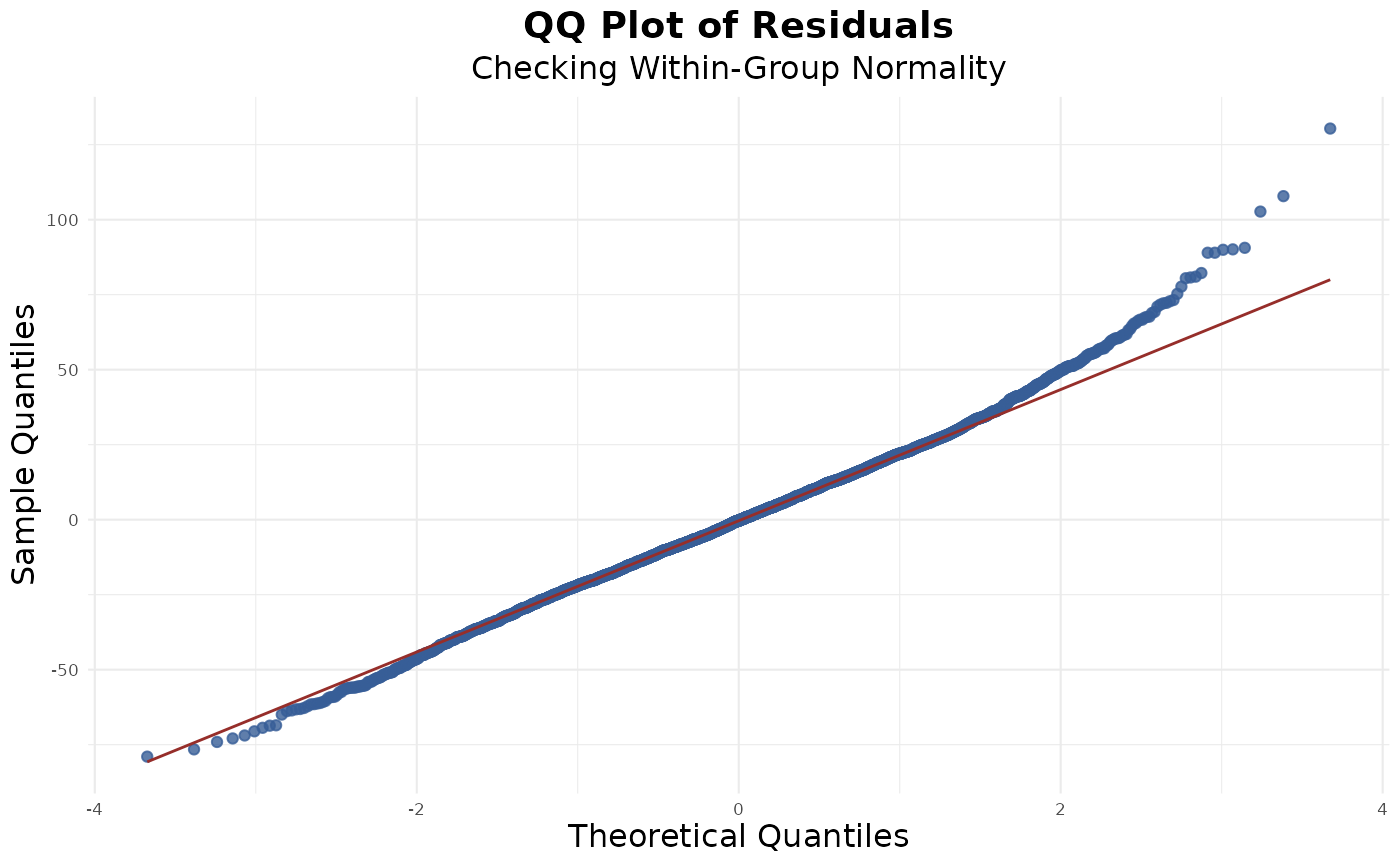

Mean-Variance Relationship

The residuals vs. fitted plot does not exhibit the classic funnel-shaped pattern, suggesting that the assumption of constant variance (homoscedasticity) is reasonably met. Consider variable transformations if you do notice funneling or specific patterns:

res_fit(model)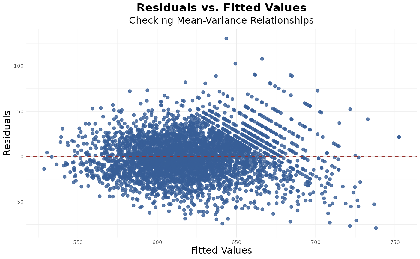

Homoscedasticity

The boxplot of residuals by school shows relatively consistent spread across most groups, suggesting that the assumption of equal residual variance within groups is reasonably satisfied:

res_box(model, group_var = "school_id")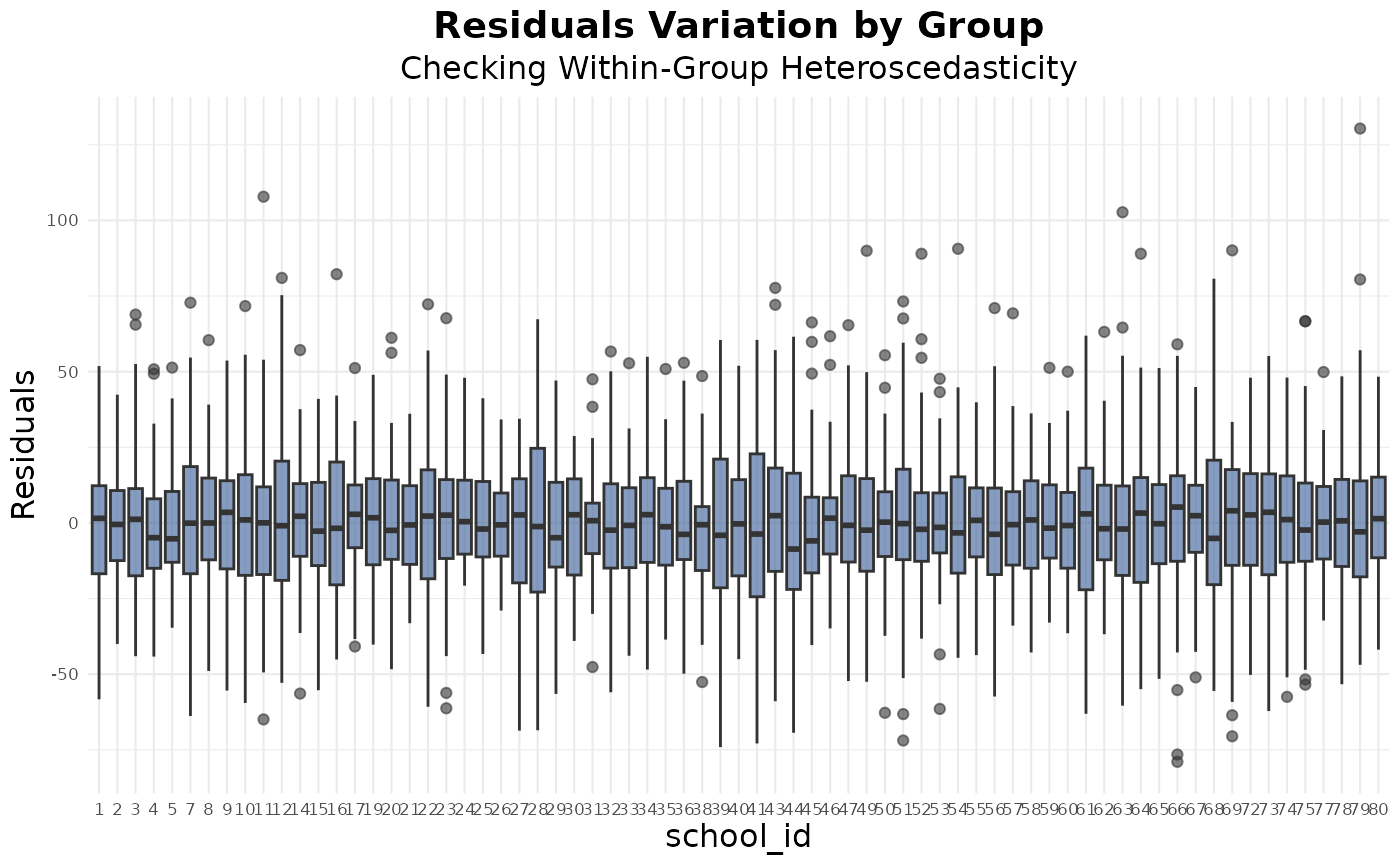

Testing Effects

Once you’ve interpreted your model and checked that assumptions reasonably hold, the next natural step is to test whether certain effects — fixed or random — meaningfully contribute to your model. lrt_lmer() provides likelihood ratio tests on a selected fixed or random effect in a fitted lme4::lmer() model. It aims to gauge the effect brought in by one single term and apply statistically accurate null distribution based on different effect types.

Depending on whether you’re testing a fixed effect or a random effect by the type argument, the structure of the reduced model differs. Currently, the function only supports lmer models with fixed effects and a single random structure (i.e., no nested /, double vertical ||, or multi-level random effects). To see more about the testing logic and how the reduced models are constructed differently, run ?lrt_lmer.

Fixed Effects

To test whether a selected fixed effect exists, specify the exact variable name in target and set type = "fixed". This will allow the function to match with the underlying set of fixed terms. Running the function will give a summary of output, along with the test statistics being returned as a list:

fix_result <- lrt_lmer(model, target = "math_old", type = "fixed", data = star)
#> Likelihood Ratio Test for 'math_old' (fixed effect)
#> Full Model: math ~ cltype + math_old + (cltype | school_id)
#> Reduced Model: math ~ cltype + (cltype | school_id)
#> Test Statistics:
#> - Log-Likelihood Difference: 3202.807
#> - Degrees of Freedom: 1 (Difference in estimated parameters)
#> - P-Value: < 2.2e-16 (Chi-square test)
#> Since p = < 2.2e-16, under alpha level of 0.05, we reject the null hypothesis. The test suggests that the fixed effect of math_old is statistically significant and contributes to the model.

fix_result
#> $logLik
#> [1] 3202.807
#> 
#> $df
#> [1] 1
#> 
#> $pvalue
#> [1] 0

NOTE: If interaction is fitted to the model, specify has_interaction = TRUE in the input argument. The reduced model will be subsequently constructed without the selected fixed effect and any interaction terms containing it.

Random Effects

To test the excess heterogeneity contributed by a random effect term, specify the exact variable name in target and set type = "random". Then, the function will check whether the target is a random intercept (grouping variable) or a random slope in the model, and apply corresponding computation for the likelihood ratio test.

Random Intercept: The full model is reconstructed by modifying the original lme4::lmer() call to retain only the random intercept (ignoring any random slopes). The reduced model is a standard stats::lm() model containing only the fixed effects, and the likelihood ratio test follows a mixture Chi-square distribution for p-value computation.

random_result1 <- lrt_lmer(model, target = "school_id", type = "random", data = star)
#> Likelihood Ratio Test for 'school_id' (random intercept effect)
#> Full Model: math ~ cltype + math_old + (1 | school_id)
#> Reduced Model: math ~ cltype + math_old
#> Test Statistics:
#> - Log-Likelihood Difference: 603.7954
#> - Degrees of Freedom: 1 (Difference in estimated parameters)
#> - P-Value: < 2.2e-16 (Chi-square test)
#> Since p = < 2.2e-16, under alpha level of 0.05, we reject the null hypothesis. The test suggests that the random intercept effect of school_id is statistically significant and contributes to the model.

Random Slope: The target variable is only removed from the random slope structure. The reduced model remains an lme4::lmer() model, and the likelihood ratio test follows a mixture Chi-square distribution for p-value computation.

random_result2 <- lrt_lmer(model, target = "cltype", type = "random", data = star)
#> Likelihood Ratio Test for 'cltype' (random slope effect)
#> Full Model: math ~ cltype + math_old + (cltype | school_id)
#> Reduced Model: math ~ cltype + math_old + (1 | school_id)
#> Test Statistics:
#> - Log-Likelihood Difference: 326.1249
#> - Degrees of Freedom: 5 (Difference in estimated parameters)
#> - P-Value: < 2.2e-16 (Chi-square test)
#> Since p = < 2.2e-16, under alpha level of 0.05, we reject the null hypothesis. The test suggests that the random slope effect of cltype is statistically significant and contributes to the model.